2022. 3. 12. 13:56ㆍTool/TensorFlow
You have learned about tensors, variables, gradient tape, and modules. In this guide, you will fit these all together to train models.
import tensorflow as tf
import matplotlib.pyplot as plt
Solving machine learning problems
Solving a machine learning problem usually consists of the following steps:
- Obtain training data
- Define the model
- Define a loss function
- Run through the training data, calculating loss from the ideal value
- Caculate gradients for that loss and use an optimizer to adjust the variables to fit the data
- Evaluate your results
Data
Each input of your data, in TensorFlow, is most always represented by a tensor, and is often a vector. In supervised training, the output is also a vector.
NUM_EXAMPLES = 201

# actual line
def f(x):
    return 3.0 * x + 2.0

# input x
x = tf.linspace(-2, 2, NUM_EXAMPLES)
x = tf.cast(x, tf.float32)

# input y
noise = tf.random.normal(shape=[NUM_EXAMPLES])
y = f(x) + noise
Model
Use tf.Variable to represent all weights in a model. Use tf.Module to encapsulate the variables and the computation.
class MyModel(tf.Module):
    def __init__(self, **kwargs):

        self.w = tf.Variable(5.0)
        self.b = tf.Variable(0.0)

    def __call__(self, x):

        return self.w * x + self.b

my_model = MyModel()

print('Variables: ')
for var in my_model.variables:
    print(var)

print('Model result: ', my_model(3.0))
Variables:
<tf.Variable 'Variable:0' shape=() dtype=float32, numpy=0.0>
<tf.Variable 'Variable:0' shape=() dtype=float32, numpy=5.0>
Model result: tf.Tensor(15.0, shape=(), dtype=float32)Loss function
A loss function measures how well the output of a model for a given input matches the target output.
def loss(t, y):
    return tf.reduce_mean(tf.square(t - y))
Training loop
Training loop consist of repeatedly doing four tasks in order:
- Generate outputs from inputs through model
- Calcuate the loss
- Find gradient by gradient tape
- Opimize variable by gradient
def train(model, x, y):

    with tf.GradientTape() as tape:
        current_loss = loss(y, model(x))

    dw, db = tape.gradient(current_loss, [model.w, model.b])

    model.w.assign_sub(0.1 * dw)
    model.b.assign_sub(0.1 * db)
    return current_loss
Train
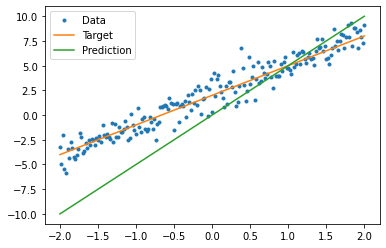
# Before
plt.plot(x, y, '.', label="Data")
plt.plot(x, f(x), label="Target")
plt.plot(x, my_model(x), label="Prediction")
plt.legend()
plt.show()
# training

weights = []
biases = []
epochs = range(10)

def report(model, loss):
    return f"W = {model.w.numpy():1.2f}, b = {model.b.numpy():1.2f}, loss={loss:2.5f}"

def training_loop(model, x, y):
    for epoch in epochs:
        current_loss = train(model, x, y)

        print(f'Epoch: {epoch:2d}: ')
        print('    ', report(model, current_loss))


current_loss = loss(y, my_model(x))

print(f'Starting:')
print('    ', report(my_model, current_loss))

training_loop(my_model, x, y)
Starting:
W = 3.15, b = 1.95, loss=0.94178
Epoch: 0:
W = 3.14, b = 1.98, loss=0.94178
Epoch: 1:
W = 3.13, b = 2.01, loss=0.93310
Epoch: 2:
W = 3.13, b = 2.02, loss=0.92767
Epoch: 3:
W = 3.12, b = 2.04, loss=0.92426
Epoch: 4:
W = 3.12, b = 2.05, loss=0.92212
Epoch: 5:
W = 3.12, b = 2.06, loss=0.92076
Epoch: 6:
W = 3.12, b = 2.07, loss=0.91991
Epoch: 7:
W = 3.11, b = 2.07, loss=0.91937
Epoch: 8:
W = 3.11, b = 2.08, loss=0.91902
Epoch: 9:
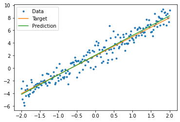
W = 3.11, b = 2.08, loss=0.91880# After
plt.plot(x, y, '.', label="Data")
plt.plot(x, f(x), label="Target")
plt.plot(x, my_model(x), label="Prediction")
plt.legend()
plt.show()
Same solution by Keras
It's useful to construct the code above with the equivalent in Keras .
Defining the model looks exactly same if you subclass tf.keras.Model. Remember that Keras models inherit ulimately from module.
class KerasModel(tf.keras.Model):
    def __init__(self, **kwargs):
        super().__init__(**kwargs)

        self.w = tf.Variable(5.0)
        self.b = tf.Variable(0.0)

    def call(self, x):
        return self.w * x + self.b

keras_model = KerasModel()
training_loop(keras_model, x, y)
keras_model.save_weights('keras_model')Epoch: 0:
W = 4.49, b = 0.42, loss=10.12811
Epoch: 1:
W = 4.12, b = 0.76, loss=6.30231
Epoch: 2:
W = 3.85, b = 1.02, loss=4.09167
Epoch: 3:
W = 3.65, b = 1.24, loss=2.80385
Epoch: 4:
W = 3.50, b = 1.41, loss=2.04744
Epoch: 5:
W = 3.40, b = 1.55, loss=1.59954
Epoch: 6:
W = 3.32, b = 1.66, loss=1.33220
Epoch: 7:
W = 3.26, b = 1.75, loss=1.17143
Epoch: 8:
W = 3.22, b = 1.82, loss=1.07404
Epoch: 9:
W = 3.19, b = 1.87, loss=1.01465You can use the built-in features of Keras as a shortcut.
If you do, you will need to use model.compile() to get the parameters, and model.fit() to train.
Keras fit expects batched data or a complete dataset as a NumPy array.
keras_model.compile(
    run_eagerly=False,
    optimizer=tf.keras.optimizers.SGD(learning_rate=0.1),
    loss=tf.keras.losses.mean_squared_error,
)

keras_model.fit(x, y, epochs=10, batch_size=1000)
Epoch 1/10
1/1 [==============================] - 0s 312ms/step - loss: 0.9782
Epoch 2/10
1/1 [==============================] - 0s 6ms/step - loss: 0.9557
Epoch 3/10
1/1 [==============================] - 0s 7ms/step - loss: 0.9418
Epoch 4/10
1/1 [==============================] - 0s 7ms/step - loss: 0.9331
Epoch 5/10
1/1 [==============================] - 0s 9ms/step - loss: 0.9277
Epoch 6/10
1/1 [==============================] - 0s 9ms/step - loss: 0.9243
Epoch 7/10
1/1 [==============================] - 0s 11ms/step - loss: 0.9221
Epoch 8/10
1/1 [==============================] - 0s 12ms/step - loss: 0.9208
Epoch 9/10
1/1 [==============================] - 0s 11ms/step - loss: 0.9199
Epoch 10/10
1/1 [==============================] - 0s 11ms/step - loss: 0.9194
<keras.callbacks.History at 0x2239dc14288>'Tool > TensorFlow' 카테고리의 다른 글
| 5. Introduction to modules, layers, and models (0) | 2022.03.12 |
|---|---|
| 4. Introduction to graphs and tf.function (0) | 2022.03.12 |
| 3. Introduction to gradients and automatic differentiation (0) | 2022.03.12 |
| 2. Introduction to Variables (0) | 2022.03.12 |
| 1. Introduction to Tensors (0) | 2022.03.12 |