2023. 9. 19. 14:36ㆍPaper Review
1. Introduction
대부분의 경우, 모델을 학습시킬 때 제한된 컴퓨팅 자원(=GPU 개수 및 기간)을 지원받는다.
그렇기 때문에, 제한된 컴퓨팅 자원에서 학습 가능한 최적의 파라미터 개수를 파악하는 것은 매우 중요한 문제다.
Kaplan는 처음으로 파라미터 개수와 모델 성능 간의 관계가 power-law임을 보였다. 이에 영향을 받아 최근에는 컴퓨팅 자원이 증가하면 토큰 개수는 거의 고정(=300B)채 모델 크기만 증가시키는 방향으로 모델들은 학습시키고 있다.
이번 연구에서는 한정된 FLOPs 지원이 주어졌을 때, 최적의 모델 크기와 토큰 개수는 무엇인지 살펴볼 것이다. (여기서 토큰 개수란 학습 도중에 본 토큰 개수를 의미한다. 즉, 같은 토큰을 또 봐도 카운트한다.)
(이 연구는, 한정된 D (or M)에서 최적 혹은 가성비 좋은 M (or D)을 조사하는 연구가 아니다!!)
이를 수식화 하면 다음과 같습니다.
$$N_{opt}(C), D_{opt}(C) = \arg \min_{\text{N, D, s.t. FLOPs(N, D)=C}} \text{L(N, D)}$$
제한된 컴퓨팅 자원(C=FLOPs(N, D))가 주어졌을 때, 손실 값(L(N, D))을 최소화하는 N, D($N_{opt}$, $D_{opt}$)를 찾는 공식이다.
모델 크기(70M ~ 16B)와 토큰 개수(5B ~ 400B)가 다른 400개의 모델을 학습시켜 위 함수(($N_{opt}$, $D_{opt}$))를 추정할 것이다.
이 결과로 Gopher에 사용된 컴퓨팅 자원의 최적 파라미터 개수와 최적 토큰 개수를 예측해본 결과, 모델 크기는 4배 작고, 토큰 개수는 4배 커야한다는 결과가 나왔다. 이를 검증하기 위해, Chinchilla 모델(크기=70B, 토큰=1.4T)을 만들었다.
학습한 결과, Chinchilla는 Gopher보다 좋은 성능을 보여줬다.
In practice, the allocated training compute budget is often known in advance: how many accelerators are available and for how long we want to use them. Since it is typically only feasible to train these large models once, accurately estimating the best model hyperparameters for a given compute budget is critical.
Kaplan et al. (2020) showed that there is a power law relationship between the number of parameters in an autoregressive language model (LM) and its performance.
One notable conclusion in Kaplan et al. (2020) is that large models should not be trained to their lowest possible loss to be compute optimal. Whilst we reach the same conclusion, we estimate that large models should be trained for many more training tokens than recommended by the authors.
we find that model size and the number of training tokens should be scaled in equal proportions.
many of the recently trained large models have been trained for approximately 300 billion tokens, in line with the approach of predominantly increasing model size when increasing compute.
Given a fixed FLOPs budget, how should one trade-off model size and the number of training tokens?
To answer this question, we model the final pre-training loss L(N, D) as a function of the number of model parameters N, and the number of training tokens, D. Since the computational budget C is a deterministic function FLOPs(N, D) of the number of seen training tokens and model parameters, we are interested in minimizing L under the constraint FLOPs(N, D)=C:
$$N_{opt}(C), D_{opt}(C) = \arg \min_{\text{N, D, s.t. FLOPs(N, D)=C}} \text{L(N, D)}$$
The functions $N_{opt}(C)$ and $D_{opt}$ describe the optimal allocation of a computational budget. We empirically estimate these functions based on the losses of over 400 models, ranging from under 70M to over 16B parameters, and trained on 5B to over 400B tokens.
Based on our estimated compute-optimal frontier, we predict that for the compute budget used to train Gopher, an optimal model should be 4 times smaller, while being training on 4 times more tokens. We verify this by training a more compute-optimal 70B model, called Chinchilla, on 1.4 trillion tokens. Not only does Chinchilla outperform its much larger counterpart, Gopher, but its reduced model size reduces inference cost considerably and greatly facilitates downstream uses on smaller hardware.
2. Related Work
1. 대규모 언어 모델
언어 모델 크기 증가는 수많은 task의 SOTA 성능을 향상시켰다. 그럼에도 불구하고, LLM은 압도적인 컴퓨팅 자원과 양질의 데이터가 필요하다는 한계점이 있다. 참고로, 이번 연구에서는, 양질의 데이터가 모델 크기를 증가시키는데 무조건 필요한 요소임을 보였다.
2. 확장(모델 크기 or 토큰 개수) 모델링
언어 모델의 확장 방식과 그로 인한 특성(성질) 변화를 이해하는 것은 거대 모델을 개발할 때 중요하다.
kaplan은 처음으로 모델 크기와 손실값 간의 관계가 pwer-law임을 보였다. 이번 연구에서는, 한정된 컴퓨팅 자원에서 학습시킬 수 있는 최적의 모델 크기에 대해 조사할 것이다.
우리와 kaplan 간의 차이점은 2가지다. 1). kaplan은 토큰 개수와 학습률을 고정했다. 즉, 이들과 loss 간의 관계를 파악하지 않았다. 그에 반해, 우리는 토큰 개수에 따라 학습률을 적절히 설정하는 것이 최소 손실값을 가져온다는 것을 보였다.
2). 우리는 500M ~ 16B 크기의 모델까지 학습시켜, 계산량과 손실값 간의 관계를 관찰했다. 하지만, kaplan이 학습시킨 모델은 100M 크기의 모델로 우리에 비해 작다
최근에는, Clark가 MoE 크기 확장에 따른 성질 변화를 관찰했다. 모델 크기 확장에 따른 expert 확장성은 감소된다. 이 접근법은 모델 크기와 expert 개수로 손실을 모델링했다. 하지만 이들도, 토큰 개수를 고정했다.
3. 거대 모델에 맞는 하이퍼 파리미터 조사
모델 크기와 토크 개수 뿐만 아니라, 다른 하이퍼 파리미터(학습률, 배치 크기, 옵티마이저, 깊이-넓이 비율)도 중요한 요소다.
이번 연구에서는, 모델 크기와 step 횟수에 집중을 할 것이다. 나머지 하이퍼 파리미터는 이전 연구를 참조할 것이다.
1). Yang은 트렌스포머의 다양한 하이퍼 파라미터의 선택 방법을 연구했다. 2). McCandilish은 배치 크기와 모델 크기 간의 상관관계를 파악했다. 3). Zhang은 기존보다 더 큰 배치 크기 사용이 가능함을 보였다. 4). Levine은 여러 모델 크기에서 최적의 깊이-넓이 비율을 조사했다.
4. 향상된 모델 구조
최근에 기존 트렌스포머의 대안들이 나오고 있다. 예를 들어, 1). MoE(Mixture of Expert)는 조건부 연산을 통해 학습 및 추론 연산 비용이 낮춰 크지만 효율적인 모델을 제공한다. 하지만, 모델이 매우 클 경우 이러한 연산 이점은 큰 의미가 없어보인다. 2). 트랜스포머와 보상 방식을 합쳐 언어 모델을 향상시킨 방식도 나왔다. 이 방식은 학습 때, 볼 수 있는 토큰 개수를 증가시켜준다. 이는 언어 모델의 성능이 이전에 생각했던거보다 토큰 개수에 더 영향을 받음(민감함)을 시사한다.
Large language models.
increasing the size of language models has been responsible for improving the state-of-the-art in many language modelling tasks. Nonetheless, large language models face several challenges, including their overwhelming computational requirements and the needs for acquiring more high-quality training data. In fact, in this work we find that larger, high quality datasets will play a key role in any further scaling of language models.
Modelling the scaling behavior.
Understanding the scaling behaviour of language models and their transfer properties has been important in the development of recent large models. Kaplan first showed a predictable relationship between model size and loss over many orders of magnitude. The authors investigate the question of choosing the optimal model size to train for a given compute budget.
Our work differs from Kaplan in several important ways. First the authors use a fixed number of training tokens and learning rate schedule for all models; this prevents them from modelling the impact of these hyperparameters on the loss. In contrast, we find that setting the learning rate schedule to approximately match the number of training tokens results in the best final loss regardless of model size.
Secondly, we include models with up to 16B parameters, as we observe that there is slight curvature in the FLOP-loss frontier - in fact, the majority of the models used in our analysis have more than 500 million parameters, in contrast the majority of runs in kaplan are significantly smaller - many being less than 100M parameters.
Recently, Clark specifically looked in to the scaling properties of Mixture of Expert language models, showing that the scaling with number of experts diminishes as the model size increases - their approach models the loss as a function of two variables: the model size and the number of experts. However, the analysis is done with a fixed number of training tokens.
Estimating hyperparameters for large models.
Other important factors include learning rate, learning rate schedule, batch size, optimiser, and width-to-depth ratio.
In this work, we focus on model size and the number of training steps, and we rely on existing work and provided experimental heuristics to determine the other necessary hyperparameters.
Yang investigates how to choose a variety of these parameters for training an autoregressive transformer, including the learning rate and batch size. Zhang suggest that using larger batch-sizes than those we use is possible. Levine investigates the optimal depth-to-width ratio for a variety of standard model sizes.
Improved model architectures.
Recently, various promising alternatives to traditional dense transformers have been proposed. For example, through the use of conditional computation large MoE models are able to provide a large effective model size despite using relatively fewer training and inference FLOPs. However, for very large models the computational benefits of routed models seems to diminish. An orthogonal approach to improving language model is to augment transformers with explicit retrieval mechanisms.
This approach effectively increases the number of data tokens seen during training. This suggests that performance of language models may be more dependant on the size of the training data than previously thought.
3. Estimating the optimal parameter / training tokens allocation
세 가지 접근법으로 한정된 컴퓨팅 자원에서의 최적 파라미터 개수와 토큰 개수를 파악해볼 것이다.
우선 모델 크기(70M ~ 16B)와 토큰 개수(5B ~ 400B)가 다른 400개의 모델을 학습시킨 후, 그 결과로 그 이상의 컴퓨팅 자원에서의 최적 파라미터 개수와 토큰 개수를 유추해볼 것이다. 이때, 우리는 컴퓨팅 자원과 모델 크기가 power-law 관계를 가진다고 가정할 것이다.
세 가지 접근법 모두 모델 크기 증가율과 토큰 개수 증가율이 동일해야 한다는 실험 결과를 내보였다.
We present three different approaches to answer the question driving our research: Given a fixed FLOPs budget, how should one trade-off model size and the number of training tokens? In all three case we start by training a range of models varying both model size and the number of training tokens and use the resulting training curves to fit an empirical estimator of how they should scale.
We assume a power-law relationship between compute and model size as done in Clart; Kaplan, through future work may want to include potential curvature in this relationship for large model sizes. The resulting predictions are similar for all three methods and suggest that parameter count and number of training tokens should be increased equally with more compute.
3.1. Approach 1: Fix model sizes and vary number of training tokens
첫 접근법에서는 각 모델 크기마다 서로 다른 네 가지 step 개수 (or 토큰 개수)를 사용해 네 개 모델을 학습시켰다.
이때, 네 개 모델을 학습시킬 때, lr decay를 10x로 설정하고, 토큰 개수를 최대 16x까지 달리한다. (e.g., 1x, 4x, 8x, 16x)
(토큰 혹은 step 개수가 많아지면, cosine cycle length를 높여 천천히 감소시킨다.)
이를 통해, 각 모델의 FLOP와 loss 간의 관계를 수집할 수 있을 뿐만 아니라, 각 FLOP의 최소 loss를 갖는 모델 크기와 토큰 개수 조합을 찾을 수 있다.
이렇게 수집한 데이터를 활용해, FLOP에서 최적 파라미터 개수와 토큰 개수를 매핑하는 함수를 근사할 수 있다. 참고로, 관계가 power-law를 따른다고 가정했다.

실험 결과는 다음과 같다. $N_{opt} \propto C^{0.5}$, $D_{opt} \propto C^{0.5}$
we vary the number of training steps for a fixed family of models (ranging from 70M to over 16B parameters), training each model for 4 different number of training sequences.
For each parameter count N we train 4 different models, decaying the learning rate by a factor of 10x over a horizon (measured in number of training tokens) that ranges by a factor of 16x.
(In all cases, the learning rate drops by a factor of 10x during training, using cosine schedule.)
We make the assumption that the cosine cycle length should be approximately matched to the number of training steps.
From this, we obtain a continuous mapping from FLOP count to training loss for each run. Then, for each FLOP count, we determine which run achieves the lowest loss. Using these interpolants, we obtain a mapping from anyFLOP count C, to the most efficient choice of model size N and number of training tokens D such that FLOPs(N, D) = C.
Finally, we fit powers laws to estimate the optimal model size and number of training tokens for any given amount of compute.
We find that a = 0.50 and b =0.50.
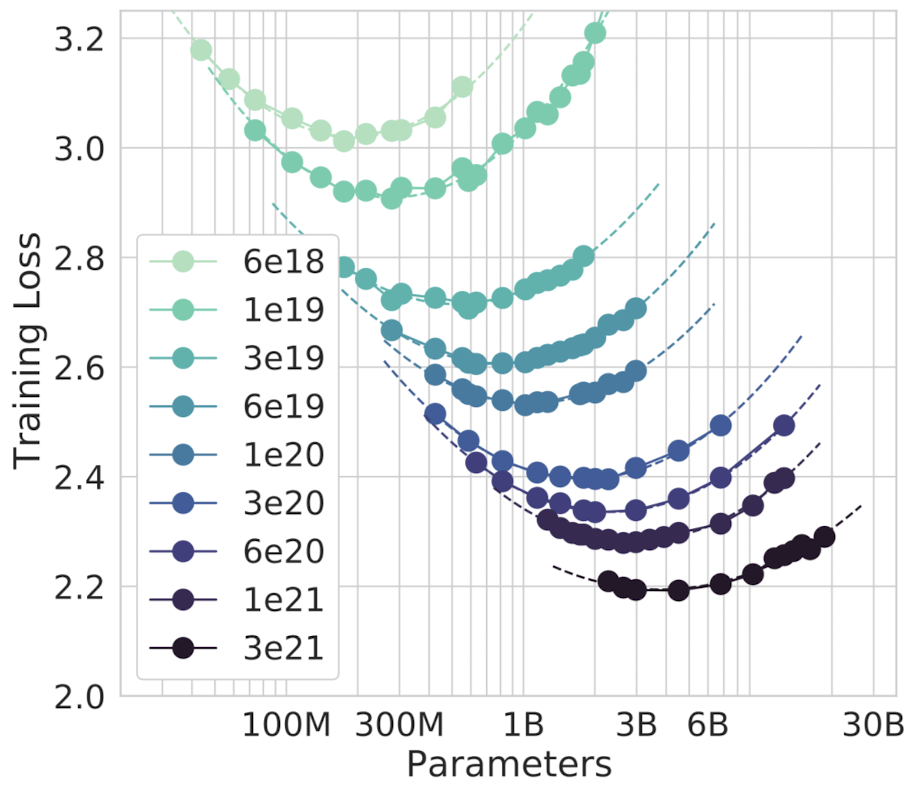
3.2. Approach 2: IsoFLOP profiles
두번째 접근법에서는 모든 모델 크기를 학습시켰다. 이때, 9개의 FLOPs를 선정하고, 각 FLOPs의 최종 loss값을 측정했다.
참고로, 토큰 개수는 모델 크기와 FLOPs를 고려해서 결정했다.
이를 통해, 각 FLOP에서 loss값이 가장 낮은 모델 크기가 무엇인지 바로 파악할 수 있다.
(각 FLOP 마다 포물선을 그려, 최소 loss값을 갖는 모델 크기를 빠르게 파악했다.)
이전 접근법과 마찬가지로, FLOP와 최적 파라미터 개수 간의 관계가 power-law를 따른다고 가정했다.
실험 결과는 다음과 같다. $N_{opt} \propto C^{0.49}$, $D_{opt} \propto C^{0.51}$
In our second approach we vary the model size for a fixed set of 9 different training FLOP counts, and consider the final training loss for each point.
This allows us to directly answer the question: For a given FLOP budget, what is the optimal parameter count?
We fit a parabola to each IsoFLOPs curve to directly estimate at what model size the minimium loss is achieved.
As with the previous approach, we then fit a power low between FLOPs and loss-optimal model size and number of training tokens.
we find that a = 0.49 and b= 0.51.
3.3. Approach 3: Fitting a parametric loss function
마지막 접근법은 loss값을 파라미터 개수와 토큰 개수로 모델링했다.
$$\hat L(N, D) \triangleq E = \frac{A}{N^\alpha} + \frac{B}{D^\beta}$$
첫번째 항은 데이터 분포에 대한 이상적인 생성 프로세스의 loss값을 의미한다.
두번째 항은 트렌스포머와 이상적인 생성 프로세스 간의 성능 차이를 의미한다.
(즉, 완벽하게 학습된 트렌스포머도 이상적인 생성 프로세스보다 성능이 낮다.)
세번째 항은 샘플링된 데이터만으로 유한번의 최적화 학습을 진행하여 발생한 수렴값과의 차이를 의미한다.
Model fitting
(A, B, E, $\alpha$, $\beta$)을 추정하기 위해, L-BFGS 알고리즘으로 Huber loss(=예측 loss와 실제 loss 간의 차이)를 최소화해야 한다.
$$\min_{A, B, E, \alpha, \beta} \sum_{\text{Runs }i} \text{Huber}_\gamma \left( \log \hat L(N, D) - \log L_i \right)$$
참고로, Huber loss는 이상치 예측 성능이 좋다.
Efficient frontier
FLOPs(N, D) $\sim$ 6ND 제약 조건 하에서, $\hat L(N, D)$을 최소화하여 $N_{opt}$ and $D_{opt}$을 근사할 수 있다.
$\hat L(N, D)$의 최소화 조건은 $\frac{A}{N^\alpha} = \frac{B}{D^\beta}$이므로, power-law로 $N_{opt}$과 $D_{opt}$을 다음과 같이 근사할 수 있다.
$$N_{opt}(C) = G\frac{C}{6}^a, \quad D_{opt}(C) = G^{-1}G\frac{C}{6}^b, \quad \text{where} \quad G = \left(\frac{\alpha A}{\beta B}\right)^\frac{1}{\alpha + \beta}, \quad a = \frac{\beta}{\alpha + \beta}, \quad b = \frac{\alpha}{\alpha + \beta}$$

실험 결과는 다음과 같다. $N_{opt} \propto C^{0.46}$, $D_{opt} \propto C^{0.54}$
Lastly, we model all final losses from experiments in Approach 1 & 2 as a parametric function of model parameter count and number of seen tokens.
The first term captures the loss for a ideal generative process on the data distribution, and should correspond to the entropy of natural text. The second term captures the fact that a perfectly trained transformer with N parameters underperforms the ideal generative process. The final term captures the fact that the transformer is not trained to convergence, as we only make a finite number of optimisation steps, on a sample of the data distribution.
Model fitting. To estimate (A, B, E, $\alpha$, $\beta$), we minimize the Huber loss between the predicted and observed log loss using the L-BFGS algorithm.
$$\min_{A, B, E, \alpha, \beta} \sum_{\text{Runs }i} \text{Huber}_\gamma \left( \log \hat L(N, D) - \log L_i \right)$$
The Huber loss ($\gamma = 10^{-3}$) is robust to outliers, which we find important for good predictive performance over held-out points.
Efficient frontier. We can approximate the functions $N_{opt}$ and $D_{opt}$ by minimizing the paramatric loss $\hat L(N, D)$ under the constraint FLOPs(N, D) $\sim$ 6ND. The resulting $N_{opt}$ and $D_{opt}$ balance the two terms in Equation (3) that depend on model size and data. By construction, they have a power-law form:
$$N_{opt}(C) = G\frac{C}{6}^a, \quad D_{opt}(C) = G^{-1}G\frac{C}{6}^b, \quad \text{where} \quad G = \left(\frac{\alpha A}{\beta B}\right)^\frac{1}{\alpha + \beta}, \quad a = \frac{\beta}{\alpha + \beta}, \quad b = \frac{\alpha}{\alpha + \beta}$$
we find that a = 0.46 and b = 0.54.
3.4. Optimal model scaling
세 가지 접근법 모두 "컴퓨팅 자원이 증가하면, 모델 크기와 토큰 개수를 같은 비율로 증가시켜야 한다"고 주장한다.

표3에는 모델 크기마다 계산 최적화를 위한 FLOPs와 토큰 개수를 보여준다. 이를 통해 3가지 사실을 알 수 있다.
1). 최근 LLM들의 모델 크기가 컴퓨팅 자원에 비해 매우 크다.
2). 최근 LLM 모델 크기에서의 계산 최적화를 위해 필요한 토큰 개수가 기존 학습 토큰 개수보다 훨씬 많다. 이로 데이터 수집의 중요성을 올라갈 것이다.
3). 최근 LLM에 사용된 컴퓨팅 자원이 주어지면, 더 많은 토큰으로 더 작은 모델을 학습시켜 성능 향상을 보일 수 있다.
C4와 GitHub 코드 데이터로 모델을 학습시켜 LsoFLOP 표를 그려본 결과, "모델 크기와 토큰 개수는 같은 비율로 증가시켜야 한다는 결론이 나왔다. 즉, 위 결과는 데이터의 특징, 속성, 성질에 영향을 받지 않는다.
All three approaches suggest that as compute budget increases, model size and the amount of training data should be increased in approximately equal proportion.
In Table 3 we show that estimated number of FLOPs and tokens that would ensure that a model of a given size lies on the compute-optimal frontier. Our findings suggests that the current generation of large language models are considerably over-sized, given their respective compute budgets.
the amount of training data that is projected to be needed is far beyond what is currently used to train large models, and underscores the importance of data collection in addition to engineering improvements that allow for model scale. While there is significant uncertainty extrapolating out many orders of magnitude, our analysis clearly suggests that given the training compute budget for many current LLMs, smaller models should have been trained on more tokens to achieve the most performance model.
we reproduce the LsoFLOP analysis on two additional datasets: C4 and GitHub code. In both cases we reach the similar conclusion that model size and number of training tokens should be scaled in equal proportions.
4. Chinchilla
이전 단락에서 의하면, Gopher에 사용된 컴퓨팅 자원의 최적 파라미터 개수는 40B ~ 70B이다.
이 가설을 확인하기 위해 1.4T 개수의 토큰으로 70B 크기의 모델(=Chinchilla)을 학습시켜, Gopher를 포함한 여러 LLMs과 성능 비교를 해볼 것이다.
학습에 사용된 컴퓨팅 자원은 같지만, Chinchilla가 4x 작기 때문에, 메모리 사용량과 추론 비용이 훨씬 낮다.


Based on our analysis in Section 3, the optimal model size for the Gopher compute budget is somewhere between 40 and 70 billion parameters. We test this hypothesis by training a model on the larger end of this range - 70B parameters - for 1.4T tokens.
In this section we compare this model, which we call Chinchilla, to Gopher and other LLMs. Both Chinchilla and Gopher have been trained for the same number of FLOPs but differ in the size of the model and the number of training tokens.
Due to being 4x smaller than Gopher, both the memory footprint and inference cost of Chinchilla are also smaller.
4.1. Model and training details
Chinchilla는 Gopher와 같은 모델 구조와 훈련 설정이 거의 동일하다. 4가지 차이점이 있다. 1). 토큰 개수 증가를 고려해 Gopher와 약간 다른 학습 데이터 분포를 가지고 있다. 2). Adam 대신 AdamW 옵티마이저를 사용한다. 이는 언어 모델링 손실값을 낮춰줄 뿐만 아니라 fine-tuning 이후의 다운스트림 테스크의 성능을 향상시켜준다. 3). NFKC 정규화(=문자열 정규화)가 적용되지 않은 SentencePiece 토크나이저를 사용한다. 위 토크나이저는 Gopher 토크나이저와 94.15%로 매우 비슷하지만, 수학과 화학 표현에 도움을 준다. 4). forward, backward pass 할 때 bfloat16을 사용하지만, weight의 float32 복사본을 따로 보관한다.
Chinchilla uses the same model architecture and training setup as Gopher with the exception of the differences listed below.
we train Chinchilla on MassiveText but use a slightly different subset distribution to account for the increased number of training tokens. we use AdamW for Chinchilla rather than Adam as this improves the language modelling loss and the downstream task performance after finetuning. We train Chinchilla with a slightly modified SentencePiece tokenizer that does not apply NFKC normalization. The vocabulary is very similar - 94.15% of tokens are the same as those used for training Gopher. We find that particularly helps with the representation of mathematics and chemistry, for example. Whilst the forward and backward pass are computed in bfloat16, we store a float32 copy of the weights in the distributed optimiser state.
4.2. Results
LLMsChinchilla의 광범위하게 평가해 다른 LLMs과 비교할 것이다. (언어 모델링, 독해력, 일반 상식, 일반 추론, 유명 benchmark)

We perform an extensive evaluation of Chinchilla, comparing against various large language models.
4.2.1. Language modelling
1. Chinchilla는 The Pile의 모든 데이터셋에서 Gopher를 능가했다.
2. Chinchilla는 The Pile의 2개 데이터셋을 제외한 나머지 데이터셋에서 Jurassic-1 (178B)을 능가했다.
3.. Wikitext103에서 Chinchilla는 Gopher의 7.75ppl 대비 7.16ppl을 달성했다.
하지만, Gopher보다 4배 더 많은 데이터 사용이 test set 유출 가능성을 높여 성능을 인위적으로 향상시킬 수 있으므로, 언어 모델링 성능을 비교할 때 주의가 필요하다.
때문에, test set 유출이 덜 우려되는 다른 테스크(=MMLU, BIG-bench)에 중점을 더 둘 것이다.
Chinchilla significantly outperforms Gopher on all evaluation subsets of The Pile. Compare to Jurassic-1 (178B), Chinchilla is more performant on all but two subsets.
On Wikitext103, Chinchilla achieves a perplexity of 7.16 compared to 7.75 for Gopher. Some caution is needed when comparing Chinchilla with Gopher on these language modelling benchmarks as Chinchilla is trained on 4x more data than Gopher and thus train/test set leakage many artificially enhance the results. We thus place more emphasis on other tasks for which leakage is less of a concern, such as MMLU and BIG-bench along with various closed-book question answering and common sense analyses.
4.2.2. MMLU
MMLU는 과목 시험 형식과 비슷한 다양한 질문들로 구성되어 있다.
1. Chilchilla는 Gopher보다 훨씬 작음에도 불구하고, 평균 정확도가 7.6% 향상됐다.
2. Gopher와 비교해봤을 때, Chinchilla는 4가지 테스크를 제외한 나머지 테스크에서 같거나 높은 성능을 보였다.


The Massive Multitask Language Understanding (MMLU) benchmark consists of a range of exam-like questions on academic subjects. Chinchilla significantly outperforms Gopher despite being much smaller with an average accuracy of 67.6% (improving Gopher by 7.6%).
we find that Chinchilla improves performance on the vast majority of task. On four tasks Chinchilla underperforms Gopher, and there is no change in performance on two tasks.
4.2.3. Reading comprehension
1. 문맥의 마지막 단어를 예측하는 LAMBADA에서는, Chinchilla가 77.4% 정확도를 보였다. 참고로, Gopher와 MT-NLG는 각각 74.5%, 76.6%를 보였다.
2. RACE-h와 RAE-m에서는, Chinchilla가 Gopher 비해 정확도가 10% 이상 향상됐다.

On the final word prediction dataset LAMBADA, chinchilla achieves 77.4% accuracy, compared to 74.5% accuracy from Gopher and 76.6% from. MT-NLG 530B. On RACE-h and RACE-m, Chinchilla greatly outperforms Gopher, improving accuracy by more than 10% in both cases.
4.2.4. BIG-bench
Chilchilla는 Gopher보다 평균 정확도가 10.7% 향상돼 65.1% 정확도를 보였다.
62가지 테스크 중 오직 4가지 테스크에서는 Gopher보다 낮은 성능을 보였다.

Chinchilla outperforms Gopher on the vast majority tasks. We find that Chinchilla improves the average performance by 10.7%,reaching an accuracy of 65.1% versus 54.4% for Gopher. Of the 62 tasks we consider Chinchilla performs worse than Gopher only four.
4.2.5. Common sense
일반 추론(=상식)에서는 PIQA, SIQA, HellaSwag, BoolQ 데이터셋을 사용했다.
Chinchilla가 모든 테스크에서 Gopher와 GPT-3를 능가했다. 뿐만 아니라, 한 가지 테스크를 제외한 나머지 테스크에서 MT-NLG 530B보다 우수한 성능을 보였다.

We evaluate Chinchilla on various common sense benchmarks: PIQA, SIQA, Wingrande, HellaSwag, and BoolQ. We find that Chinchilla outperforms both Gopher and GPT-3 on all tasks and outperforms MT-NLG 530B on all but one task.
4.2.6. Closed-book question answering
1. TruthfulQA에서는, Chinchilla가 0-, 5-, 10-shot에서 43.6%, 58.5%, 66.7% 정확도를 보였다. 참고로, Gopher는 0-, 10-shot에서 29.5%와 43.7% 정확도를 보였다.
0-shot에서 14.1%의 엄청난 성능 향상은 pre-training 데이터셋의 더욱 정확한 모델링만으로도 TruthfulQA의 상당한 성능 향상을 이룰 수 있음을 시사한다.
2. Natural Question에서는 Chinchilla가 5-, 64-shot에서 31.5%, 35.5% 정확도를 달성해 closed-book SOTA에 등극했다. (참고로, Gopher는 21%와 28% 정확도를 보였다.)
3. TriviaQA에서는 필터링 버전과 필터링되지 않은 버전 모두 사용했다. 모든 버전에서 Chinchilla가 Gopher의 성능을 능가했다.
필터링된 버전에서는 Chinchilla가 open-book SOTA에 비해 오직 7.9% 뒤떨어진다. 필터링되지 않은 버전에서는 Chinchilla가 GPT-3를 능가했다.

On TruthfulQA, Chinchilla reaches 43.6%, 58.5% and 66.7% accuracy with 0-shot, 5-shot, and 10-shot respectively. In comparison, Gopher achieved only 29.5% 0-shot and 43.7% 10-shot accuracy.
The large improvement (14.1% in 0-shot accuracy) achieved by Chinchilla suggest that better modelling of the pre-training data alone can lead to substantial improvements on this benchmark.
On the Natural Questions dataset, Chinchilla achieves new closed-book SOTA accuracies: 31.5% 5-shot and 35.5% 64-shot, compared to 21% and 28% respectively, for Gopher. On TriviaQA we show results for both filtered and unfiltered set. In both cases, Chinchilla substantially out performs Gopher. On the filtered version, Chinchilla lags behind the open book SOTA by only 7.9%. On the unfiltered set, Chinchilla outperforms GPT-3.
Reading comprehension
4.2.7. Gender bias and toxicity
LLM은 공격적인 언어 사용, 사회적 편견 제시, 개인 정보 유출과 같은 잠재적 위험을 가지고 있다.
우리는 Chinchilla가 Gopher와 비슷한 위험도가 있을거라 예상한다. 같은 데이터와 비슷한 모델 구조를 사용했기 때문이다.
이번 단락에서는, 성별 (직업) 편견과 혐오 표현 생성에 대해 조사해볼 것이다.
1. 성별 편견
Winogender로 "대명사가 참조하는 직업"을 모델이 올바르게 예측할 수 있는지 평가한다. 편견이 없는 모델은 대명사의 성별과 상관없이 대명사 참조 단어를 올바르게 예측한다.
Chinchilla는 모든 집단에서 Gopher 보다 더 자주 올바르게 예측했다. 흥미롭게도, 남자 대명사(3.2%↑)가 여성 혹은 중성 대명사 (8.3%↑, 9.2%↑)에 비해 성능 향상이 낮다.
고정관념과 대조되는 gotcha로도 평가해본 결과, Chinchilla가 Gopher보다 높은 성능을 보였다.
남성/여성, gocha/not gocha로 결과를 분류해봤을 때, 여성-gocha가 가장 높은 성능 향상(10%↑)을 보였다.

비록 Chinchilla가 모든 성별 고정관념을 어느 정도 극복했지만, 성능 향상 정도가 균등하지 않다. 즉, 특정 대명사의 향상 정도가 다른 대명사보다 높다. 이는 계산 최적화를 이용해 얻은 성능 향상이 균등하지 않을 수 있음을 의미한다.
2. 혐오 표현
모델 크기 증가로 인한 언어 모델링 손실값 향상은 혐오 텍스트 생성에 영향을 거의 주지 않음을 Gopher 논문에서 보았다.
이번 연구에서는, 계산 최적화로 인한 언어 모델링 손실값 향상이 혐오 텍스트 생성에 어떤 영항을 주는지 분석해볼 것이다. 프롬프트 없이 Chinchilla로 25000개 샘플을 생성해, Gopher가 생성한 샘플과 PerspectiveAPI 혐오 점수를 비교해봤다.
실험 결과, Gopher와 Chinchilla의 혐오 점수 평균 (중앙값)은 0.081 (0.064), 0.087 (0.066)이고, 상위 5% 혐오 표현 점수는 0.230, 0.238이다.
Chinchilla의 대부분의 생성 텍스트는 혐오성이 없고, Gopher와의 혐오 정도 차이는 거의 없다. 즉, 프롬프트가 주어지지 않는 경우, 모델 손실값이 혐오 정도에 영향을 주지 않는다. 이는 학습 데이터를 더 잘 모델링하는 것이 혐오성 증가를 유발하지 않음을 의미한다.
Large Language Models carry potential risks such as outputting offensive language, propagating social biases, and leaking private information. We expect Chinchilla to carry risks similar to Gopher because Chinchilla is trained on the same data, albeit with slightly different relative weights, and because it has a similar architecture. Here, we examine gender bias (particularly gender and occupation bias) and generation of toxic language.
Gender bias.
Here, we test if potential gender and occupation biases manifest in unfair outcomes on coreference resolutions, using the Winogender dataset, in a zero-shot setting. Winogender tests whether a model can correctly determine if a pronoun refers to different occupation words. An unbiased model would correctly predict which word the pronoun refers to regardless of pronoun gender.
Chinchilla correctly resolves pronouns more frequently than Gopher across all groups. Interestingly, the performance increase is considerably smaller for male pronouns (increase of 3.2%) than for female or neutral pronouns (increases of 8.3% and 9.2% respectively). We also consider gotcha examples, in which the correct pronoun resolution contradicts gender stereotypes. we see that Chinchilla resolves pronouns more accurately than Gopher. When breaking up examples by male-female gender and gocha/not gocha, the largest improvement is on female gotcha examples (improvement of 10%) Thus, though Chinchila uniformly overcomes gender stereotypes for more coreference examples than Gopher, the rate of improvement is higher for some pronouns than others, suggesting that the improvements conferred by using a more compute-optimal can be uneven.
Sample toxicity.
Gopher found that improving language modelling loss by increasing the number of model parameters has only a negligible effect on toxic text generation; here we analyze whether the same holds true for a lower LM loss ahieved via more compute-optimal training.
we generate 25000 unprompted samples from Chinchilla, and compare their PerspectiveAPI toxicity score distribution to that of Gopher-Generated samples. Several summary statistics indicate an absence of major differences: the mean (median) toxicity score for Gopher is 0.081 (0.064), compared to 0.087 (0.066) for Chinchilla, and the 95th precentile scores are 0.230 for Gopher, compared to 0.238 for Chinchilla. That is , the majority of generated samples are classified as non-toxic and the difference between the models is negligible. In line with prior findings, this suggests that toxicity levels in unconditional text generation are largely independent of the model quality (measured in language modelling loss), i.e. that better models of the training dataset are not necessarily more toxic.
5. Discussion & Conclusion
토큰 개수는 고정한 채 모델 크기만 늘여 학습시키는 것이 최근 LLM 추세다.
이러한 추세 즉, 더 큰 LLM을 만드려는 경쟁은 컴퓨팅 자원을 낭비한다고 생각한다. 즉, 한정된 컴퓨팅 자원에서 만들 수 있는 최고의 모델을 만들지 못한다고 생각한다.
우리는 400가지 학습과 3가지 접근법을 통해, 할당된 컴퓨팅 자원에서의 최적의 모델 크기와 step 개수를 유추했다.
위 실험을 통해, Gopher의 모델 크기는 사용된 컴퓨팅 자원에 비해 클 뿐만 아니라, 토큰 개수도 부족하다고 판단했다.
이를 확인하기 위해 Chinchilla를 만들어 비교해본 결과, Gopher 뿐만 아니라 다른 LLM보다 높은 성능을 보였다.
이 연구에서도 몇가지 한계점이 존재한다. 1. 학습 비용 때문에, 비교 가능한 LLM은 Chinchilla와 Gopher 밖에 없다. (뿐만 아니라, 중간 크기의 언어 모델도 없다.) 2. 컴퓨팅 자원이 높은 구간에서는 음의 곡률이 발견됐다. 즉, LLM의 최적 모델 크기를 괴대 추정했을 가능성이 있다. 3. 대부분의 모델은 1 epoch 미만으로 데이터를 학습했다.

이러한 한계점에도 불구하고, Chilchilla와 Gopher의 비교를 통해, 우리의 성능 예측이 유효함을 보여줬다. 즉, 같은 컴퓨팅 자원에서 (모델 크기와 토큰 개수를 조절해) 성능과 추론 시간 (and 메모리 사용랑) 둘 다 향상시킬 수 있음을 보여줬다.
위 결과는 데이터 수집에 더 많은 관심을 가져야함을 의미한다. 더 나아가, 양질의 데이터 수집만이 의미가 있을 것이라고 조심스롭게 예상한다.
1. 데이터가 커질수록 언어 모델링 손실값과 다운스트림 테스크 성능에 train/test set 중복이 적절히 고려됐는지 더욱 주의를 기울여 확인해야 한다. 2. 조 단위의 토큰을 학습시킬 때는 윤리와 개인 정보 문제가 발생한다. 웹에서 대규모 데이터셋을 수집할 때, 혐오 표현, 편견, 개인 정보가 포함된다. 즉, 수집할수록 이러한 정보의 양이 증가하기에, 데이터 검사의 중요도는 올라갈 것이다.
참고로, Chinchilla도 편견과 유해성이 여전히 존재하지만, 흥미롭게도, Chinchilla가 언어 모델링 손실값이 낮음에도 불구하고 Gopher보다 덜한 것 같다. LLM 성능과 유해성 간의 관계를 이해하는 것은 매우 중요한 연구 주제다.
The trend so far in large language model training has been to increase the model size, often without increasing the number of training tokens.
we hypothesis that the race to train larger and larger model is resulting in models that are substantially underperforming compared to what could be achieved with the same compute budget.
We propose three predictive approaches towards optimally setting model size and training duration, based on the outcome of over 400 training runs. All three approaches predict that Gopher is substantially over-sized estimate that for the same budget a smaller model trained on more data will perform better. We directly test this hypothesis by training Chinchilla, a 70B parameter model, and show that it outperforms Gopher and even larger models on nearly every measured evaluation task.
there are several limitations. Due to the cost of training large models, we only have two comparable training runs at large scale (Chinchilla and Gopher), and we do not have additional tests at intermediate scales. Furthermore, we observe concavity in log($N_{opt}$) at high compute budgets. This suggests that we may still be overestimating the optimal size of large models. Finally, the training runs for our analysis have all been trained on less than an epoch of data;
Despite these limitations, the comparison of Chinchilla to Gopher validates our performance predictions, that have thus enabled training a better (and more lightweight) model at the same compute budget.
our analysis suggests an increased focus on data scaling is needed. Speculatively, we expect that scaling to larger and larger datasets is only beneficial when the data is high-quality.
Larger datasets will require extra care to ensure train-test set overlap is properly accounted for, both in the language modelling loss but also downstream tasks. Finally, training for trillions of tokens introduces many ethical and privacy concerns. Large dataset scraped from the web will contain toxic language, biases, and private information.With even larger datasets being used, the quantity (if not the frequency) of such information increases, which makes dataset introspection all the more important. Chinchilla does suffer from bias and toxicity but interestingly it seems less affected than Gopher. Better understanding how performance of large language models and toxic interact is an important future research question.
We directly test this